
Toy Example - Tabularized GiGL#
Latest version of this notebook can be found on GiGL/examples/toy_visual_example/toy_example_walkthrough.ipynb
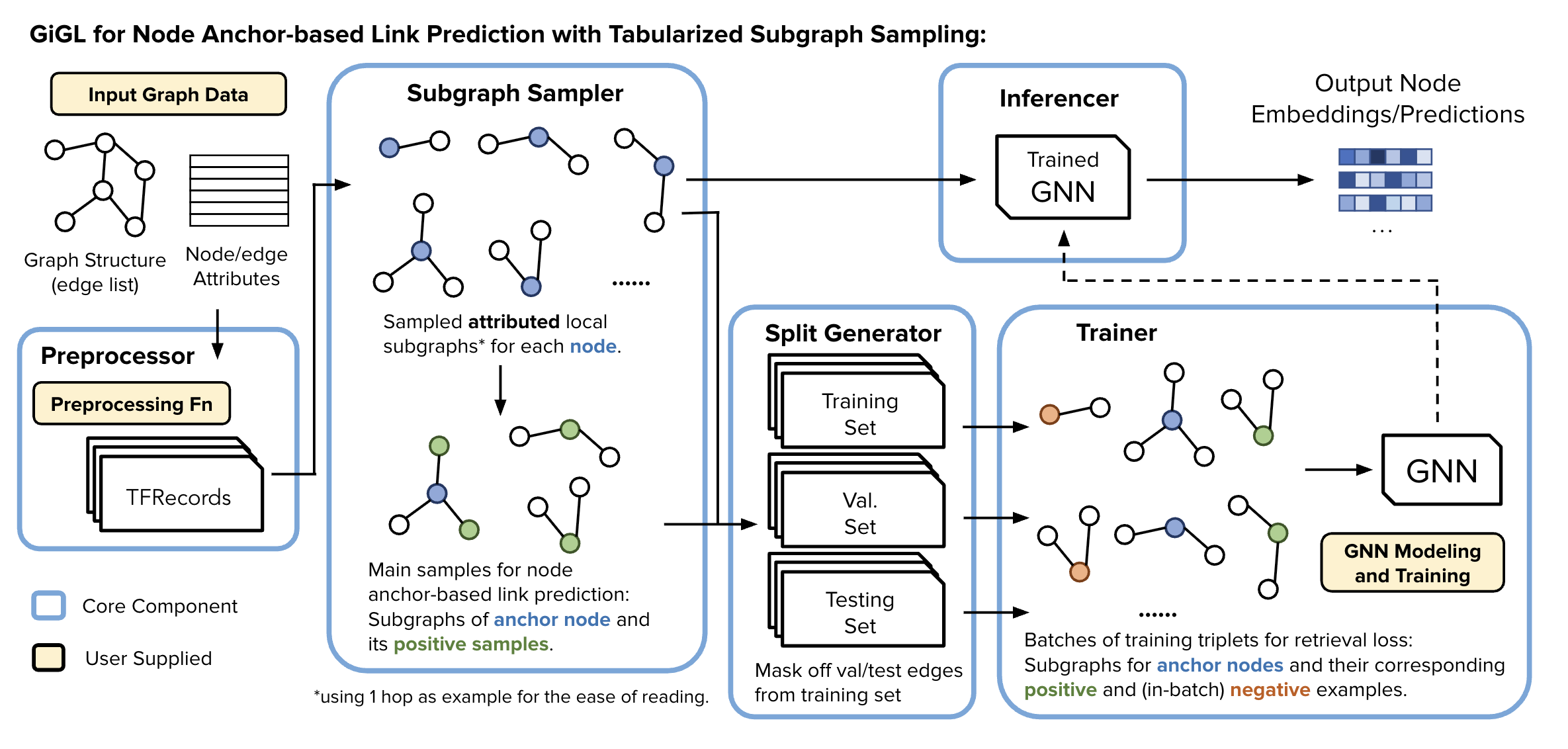
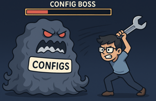
This notebook provides a walkthrough of preprocessing, subgraph sampling, and split generation components with a small toy graph for GiGL’s Tabularized setting for training/inference. It will help you understand how each of these components prepare tabularized subgraphs.
PRO TIP: you can ctrl/cmd + A, right click, then “enable scrolling for outputs”
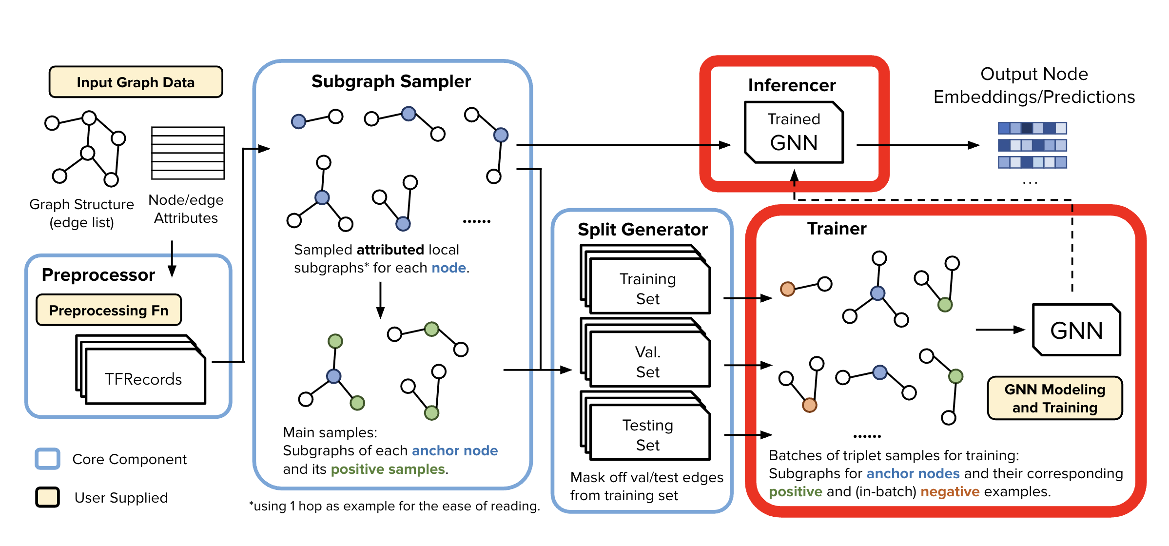
Overview Of Components#
This notebook demonstrates the process of a simple, human-digestible graph being passed through all the pipeline components in GiGL in preparation for training to help understand how each of the components work.
The pipeline consists of the following components:
📥 What You Need to Provide to GiGL#
To run your pipeline with GiGL, the user is expected to supply the following:
📊 Raw Data
Input graph data (nodes, edges, features, labels, etc.)
🛠️ Preprocessing Function
A function to specify how to transform raw data into the expected format
⚙️ Configurations
Resource Config: Specify compute and memory needs for each pipeline component
Task Config: Define modeling tasks like link prediction, node classification, etc., including sampling, GNN architecture, loss, metrics, etc.
🔁 Training & Inference Loops
User defined code that define how models are trained, validated, and used for inference
Setup Notebook#
Enabling some jupyter reload magic, reducing log clutter and changing working dir to repo root to make path resolution saner
%load_ext autoreload
%autoreload 2

import os
import pathlib

os.environ["TF_CPP_MIN_LOG_LEVEL"] = "2"  # Silence TF logspam

from gigl.common.utils.jupyter_magics import change_working_dir_to_gigl_root

change_working_dir_to_gigl_root()

NOTEBOOK_DIR = pathlib.Path(
    "./examples/toy_visual_example"
).as_posix()  # We should be in root dir because of cell # 1
Input Graph#
We use the input graph defined in examples/toy_visual_example/graph_config.yaml.
You are welcome to change this file to a custom graph of your own choosing.
Also, this is for demo purposes only; at industry-scale you probably start with a graph in some distributed datastorage layer like BigQuery
Visualizing the Input Graph#
from torch_geometric.data import HeteroData

from gigl.common.utils.jupyter_magics import GraphVisualizer, GraphVisualizerLayoutMode
from gigl.src.mocking.toy_asset_mocker import load_toy_graph

original_graph_heterodata: HeteroData = load_toy_graph(
    graph_config_path="examples/toy_visual_example/graph_config.yaml"
)  # If you want to update the graph, you will need to re-mock - See README.md


# Visualize the graph
GraphVisualizer.visualize_graph(
    original_graph_heterodata, layout_mode=GraphVisualizerLayoutMode.HOMOGENEOUS
)
✅ Validating the Configs#
You can validate both your resource and task configs using the provided tools. While the checks aren’t exhaustive, they catch the most common issues.
from gigl.src.validation_check.config_validator import kfp_validation_checks

validator = kfp_validation_checks(
    job_name=JOB_NAME,
    task_config_uri=TEMPLATE_TASK_CONFIG_PATH,
    resource_config_uri=RESOURCE_CONFIG_PATH,
    start_at="config_populator",
)
🧩 Config Populator#
The Config Populator takes a template GbmlConfig and produces a frozen GbmlConfig, where all job-related metadata paths in sharedConfig are fully populated.
These populated fields are primarily GCS paths used for communication between components—serving as intermediaries for reading and writing data. For example:
sharedConfig.trainedModelMetadatais set to a GCS URI that tells the Trainer where to write the trained model, and tells the Inferencer where to read it from.
📘 For full details, see the Config Populator Guide.
After executing the command below:
A frozen config will be created.
It will be uploaded to the
perm_assets_bucketspecified in your resource config.The resulting GCS path to the frozen config will be saved to the file defined by the
FROZEN_TASK_CONFIG_POINTER_FILE_PATHenvironment variable.
!python -m \
    gigl.src.config_populator.config_populator \
    --job_name="$JOB_NAME" \
    --template_uri="$TEMPLATE_TASK_CONFIG_PATH" \
    --resource_config_uri="$RESOURCE_CONFIG_PATH" \
    --output_file_path_frozen_gbml_config_uri="$FROZEN_TASK_CONFIG_POINTER_FILE_PATH"
🔍 Visualizing the diff between Template and the generated Frozen Config#
At this stage, we have a frozen task config, whose path is specified by the FROZEN_TASK_CONFIG_PATH environment variable. The following cell will visualize the difference between:
The original
template_task_config, andThe
frozen_task_config generatedby theconfig_populator.
📝 Note: The code in the various cells below, is solely for visualization/explanation purpses and not needed for actually working with GiGL
🔑 Key Differences#
Addition of sharedConfig:
This section contains all intermediary and final output paths required by the GiGL components (e.g., model artifacts, logs, metadata).Storage saving trick #1 - Node/Edge Type Representation Compression:
Introduces
condensedEdgeTypeMap: Maps each edge type to a unique int, where:EdgeType: Tuple[srcNodeType: str, relation: str, dstNodeType: str]EdgeType→ mapped to →int
Introduces
condensedNodeTypeMap: Maps each node type to a unique int:NodeType: strNodeType→ mapped to →int
These mappings are used to reduce storage overhead during graph processing and I/O.
ℹ️ You can provide your own condensed*Map fields, if not provided, they will be generated automatically.
from gigl.common.utils.jupyter_magics import show_task_config_colored_unified_diff

FROZEN_TASK_CONFIG_PATH: Uri
with open(FROZEN_TASK_CONFIG_POINTER_FILE_PATH.uri, "r") as file:
    FROZEN_TASK_CONFIG_PATH = UriFactory.create_uri(file.read().strip())
print(f"FROZEN_TASK_CONFIG_PATH: {FROZEN_TASK_CONFIG_PATH}")

show_task_config_colored_unified_diff(
    f1_uri=FROZEN_TASK_CONFIG_PATH,
    f2_uri=TEMPLATE_TASK_CONFIG_PATH,
    f1_name="frozen_task_config.yaml",
    f2_name="template_task_config.yaml",
)
📦 Loading the Frozen Configs#
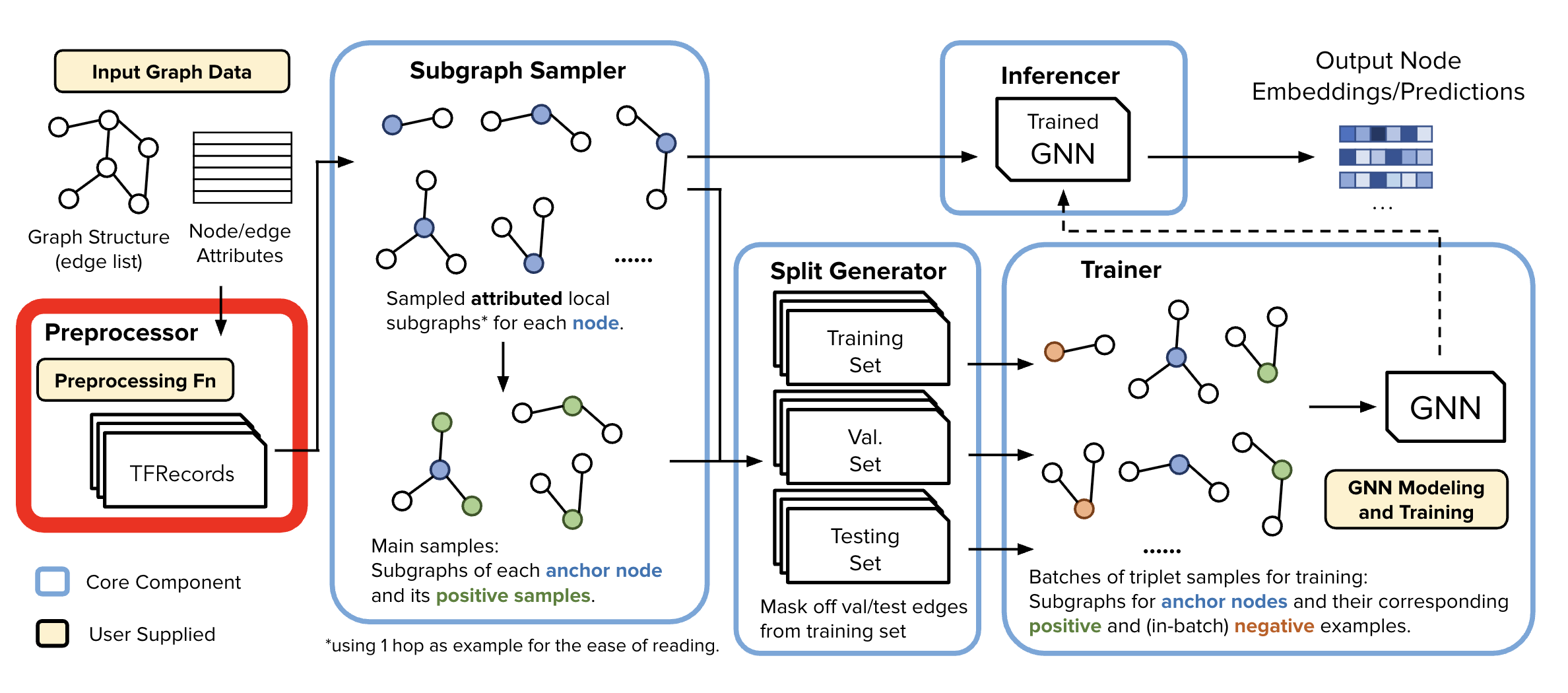
The Config Boss has been tackled - for now.
We’ll now load the frozen task and resource config files into an object so they can be referenced in the following steps.
Pro-tip: If I’ve lost you in the configs, just run all the cells.
from gigl.env.pipelines_config import get_resource_config
from gigl.src.common.types.pb_wrappers.gbml_config import GbmlConfigPbWrapper
from gigl.src.common.types.pb_wrappers.gigl_resource_config import (
    GiglResourceConfigWrapper,
)

frozen_task_config = GbmlConfigPbWrapper.get_gbml_config_pb_wrapper_from_uri(
    gbml_config_uri=FROZEN_TASK_CONFIG_PATH
)
resource_config: GiglResourceConfigWrapper = get_resource_config(
    resource_config_uri=RESOURCE_CONFIG_PATH
)
Data Preprocessor#
Once we have the configs, and our data, the first step is to preprocess the data.
Our Data Preprocessor leverages TensorFlow Transform (TFT) - which is widely used in the industry for preprocessing and feature engineering @ scale. It enables users to define data preprocessing pipelines for industry-scale data using tensorflow constructs, which can then be executed efficiently using large-scale data processing frameworks like Apache Beam.
For folks that are unfamiliar, you essentially write a function like below (with some boilerplate), and TFT will automatically create the Apache Beam computation graph so you can process TB’s of data.
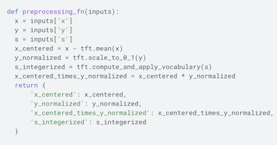
ℹ️ For this example we use toy_data_preprocessor_config.py. You will note that in this case, we are not doing anything special (i.e., no feature engineering), just reading from BQ and passing through the features.
Inputs into Data Preprocessor#
import textwrap

print("Frozen Config DataPreprocessor Information:")
print(
    "- Data Preprocessor Config: Specifies what class to use for datapreprocessing and any arguments that might be passed in at runtime to that class"
)
print(
    textwrap.indent(
        str(frozen_task_config.dataset_config.data_preprocessor_config), "\t"
    )
)
print(
    "- Preprocessed Metadata Uri: Specifies path to the preprocessed metadata file that will be generated by this component and used by subsequent components to understand and find the data that was preprocessed"
)
print(
    textwrap.indent(
        str(frozen_task_config.shared_config.preprocessed_metadata_uri), "\t"
    )
)
Running Data Preprocessor#
!python -m gigl.src.data_preprocessor.data_preprocessor \
--job_name=$JOB_NAME \
--task_config_uri=$FROZEN_TASK_CONFIG_PATH \
--resource_config_uri=$RESOURCE_CONFIG_PATH \
--custom_worker_image_uri=$DATAFLOW_RUNTIME_IMG
What is the DataPreprocessor doing?#
Node and Edge Enumeration
Applies Storage saving trick #1 - condensed edge/node type representations
Also, applies Storage saving trick #2 - Node ID Enumeration
Step to internally map all the node ids to integers to mitigate space overhead. Other components operate on these enumerated identifiers to reduce storage footprint, memory overhead, and network traffic.
Before:
NodeType: str | int | ...
NodeId: str | int | ...
EdgeType: [
    src_node_type: NodeType,
    relation: str,
    dst_node_type: NodeType
]
Edge[
    edge_type: EdgeType
    src_node: NodeId,
    dst_node: NodeId
]
After saving trick #1 and #2:
Edge[
    condensed_edge_type: int
    src_node_id: int,
    dst_node_id: int
] # 32*3 bits - wire can be even more efficient w/ batching
Apply user-defined TFT transformations
For each node and edge type, spins up a TFT Dataflow job which:
Analyzes: computes statistics from full data
Transforms: applies transformations using those statistics
Output: Transformed data to GCS
Output a Preprocessed Metadata Config
This config helps downstream components understand the data schema, types, and storage locations
In most cases, you can treat it as a black box 😮💨.
But, let’s take a quick look so you have a clearer sense of what’s inside.
frozen_task_config = GbmlConfigPbWrapper.get_gbml_config_pb_wrapper_from_uri(
    gbml_config_uri=FROZEN_TASK_CONFIG_PATH
)
preprocessed_metadata_pb = (
    frozen_task_config.preprocessed_metadata_pb_wrapper.preprocessed_metadata_pb
)
print(preprocessed_metadata_pb)
Lets also take a look at that what kind of files are generated#
print("Condensed Node Type Mapping:")
print(
    textwrap.indent(
        str(frozen_task_config.graph_metadata.condensed_node_type_map), "\t"
    )
)
print("Condensed Edge Type Mapping:")
print(
    textwrap.indent(
        str(frozen_task_config.graph_metadata.condensed_edge_type_map), "\t"
    )
)

preprocessed_nodes = (
    preprocessed_metadata_pb.condensed_node_type_to_preprocessed_metadata[
        0
    ].tfrecord_uri_prefix
)
preprocessed_edges = (
    preprocessed_metadata_pb.condensed_edge_type_to_preprocessed_metadata[
        0
    ].main_edge_info.tfrecord_uri_prefix
)
print(f"Preprocessed Nodes are stored in: {preprocessed_nodes}")
print(f"Preprocessed Edges are stored in: {preprocessed_edges}")
There is not a lot of data so we will have likely just generated one file for each of the preprocessed nodes and edges.
!gsutil ls $preprocessed_nodes && gsutil ls $preprocessed_edges
Subgraph Sampler (SGS)#
!python -m gigl.src.subgraph_sampler.subgraph_sampler \
--job_name=$JOB_NAME \
--task_config_uri=$FROZEN_TASK_CONFIG_PATH \
--resource_config_uri=$RESOURCE_CONFIG_PATH
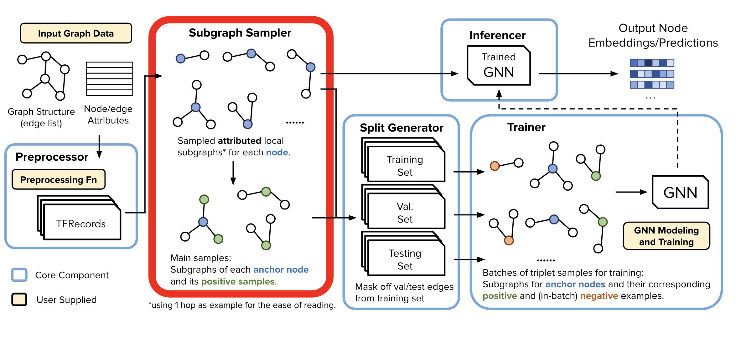
🎯 Purpose of the SGS#
Trainer memory saving trick: SGS processes node and edge data from the Data Preprocessor to generate localized training and inference samples of k-hop localized subgraphs. This design allows each of the samples to be stored independently, enabling downstream components to work efficiently with just relevant node batches—no need to load the entire graph into memory.
📁 Output Structure#
Upon completion, for this specific use case of Anchor-Based Link Prediction, SGS produces two directories of subgraph samples:
Node-Anchor-Based Link Prediction Training Samples
Generated a specified number of samples
Contains:
Root node and its sampled neighborhood w/
Positive edges, and their respective node’s sampled neighborhoods
Rooted Neighborhood Samples
Generated for each node in the graph
Contains sampled node neighborhoods
Used for both inference and as negative training samples
At, training time these are sampled randomly for each training batch
At the gigantic scale we operate in, these are almost certainly not true edges.
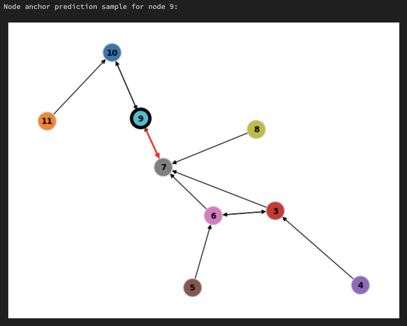
📸 Example Visualizations#
Each run of the sampler produces different subgraphs due to randomized sampling. Below are example snapshots:
Training Sample (2 hop subgraph)#
Root Node:
9Positive Edge:
9 --> 7Node
8is node9’s two hop; node2is node7’s two hop
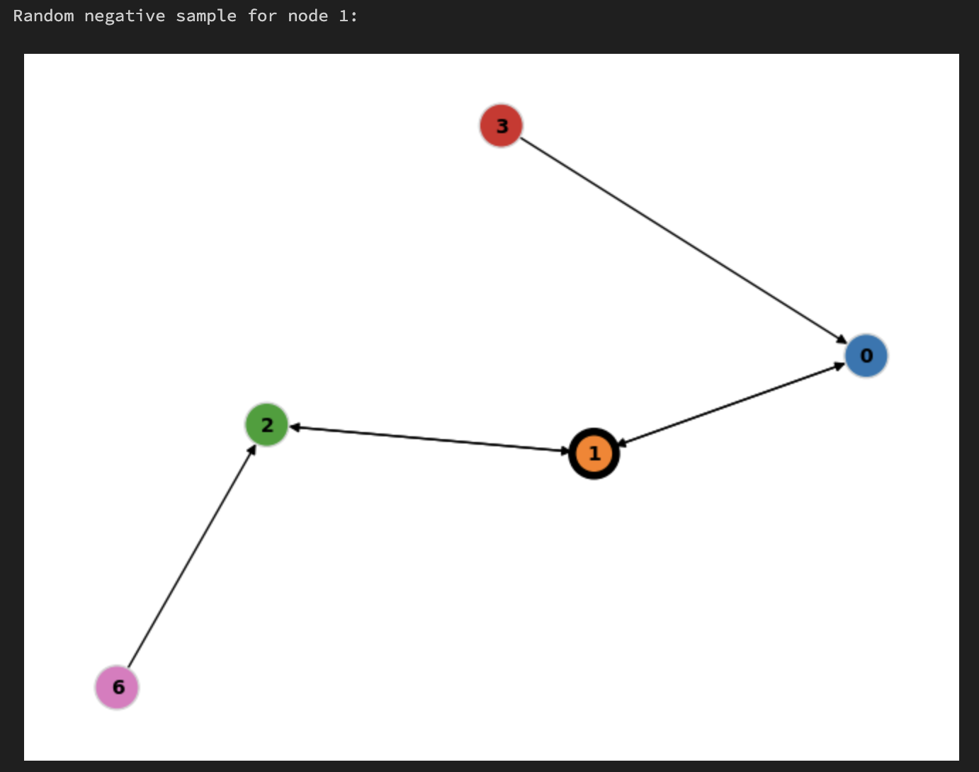
Random negative#
Root Node:
1The training data loader may choose to randomly sample any rooted node neighborhood to act as a “negative sample” - in this case it chose
1When doing inference for root node
1we will also use this subgraph
⚙️ Scalable Sample Generation with Spark#
The SGS extract-transform-load (ETL) pipeline leverages Apache Spark to perform large-scale joins required for subgraph sampling. Considerable engineering effort went into optimizing this pipeline, including:
Fine-tuning partitioning strategies
Managing data shuffling, caching, and spill behavior
Reducing unnecessary CPU overhead
This enables efficient subgraph construction without requiring a shared in-memory graph state, mirroring the data-parallel paradigm commonly used in other large-scale ML workflows.
While frameworks like GraphLearn, ByteGNN, DeepGNN, and GraphStorm rely on real-time sampling through graph backends and partition-aware execution (inspired by works from Chiang et al., Karypis, and Kumar), approaches like AGL, TF-GNN, and MultiSAGE favor tabularization—transforming graph structure into flat tables for scalable processing.
🖼️ Visualizing Samples#
We will see where the SGS data is generated below, followed by rendering a few samples and random negatives.
# Flattened Graph Metadata
flattened_graph_metadata = frozen_task_config.shared_config.flattened_graph_metadata
print(flattened_graph_metadata)

from gigl.common.utils.jupyter_magics import (
    GraphVisualizer,
    GraphVisualizerLayoutMode,
    PbVisualizer,
    PbVisualizerFromOutput,
)
from snapchat.research.gbml import training_samples_schema_pb2

# We will sample node with this id and visualize it. You will see positive edge marked in red and the root node with a black border.
SAMPLE_NODE_ID = 9
# We will sample random negative nodes with these ids and visualize them. You will see the root node with a black border.
SAMPLE_RANDOM_NEGATIVE_NODE_IDS = [1, 3]

print(f"The original global graph:")
GraphVisualizer.visualize_graph(
    original_graph_heterodata, layout_mode=GraphVisualizerLayoutMode.HOMOGENEOUS
)
pb_visualizer = PbVisualizer(frozen_task_config)
print(FROZEN_TASK_CONFIG_PATH)

print(f"Node anchor prediction sample for node {SAMPLE_NODE_ID}:")
sample = pb_visualizer.find_node_pb(
    unenumerated_node_id=SAMPLE_NODE_ID,
    unenumerated_node_type="user",
    pb_type=training_samples_schema_pb2.NodeAnchorBasedLinkPredictionSample,
    from_output=PbVisualizerFromOutput.SGS,
)
print(f"Node anchor prediction sample for node {SAMPLE_NODE_ID}:")
pb_visualizer.plot_pb(sample, layout_mode=GraphVisualizerLayoutMode.HOMOGENEOUS)

for random_negative_node_id in SAMPLE_RANDOM_NEGATIVE_NODE_IDS:
    random_negative_sample = pb_visualizer.find_node_pb(
        unenumerated_node_id=random_negative_node_id,
        unenumerated_node_type="user",
        pb_type=training_samples_schema_pb2.RootedNodeNeighborhood,
        from_output=PbVisualizerFromOutput.SGS,
    )
    print(f"Random negative sample for node {random_negative_node_id}:")
    pb_visualizer.plot_pb(
        random_negative_sample,
        layout_mode=GraphVisualizerLayoutMode.HOMOGENEOUS,
    )
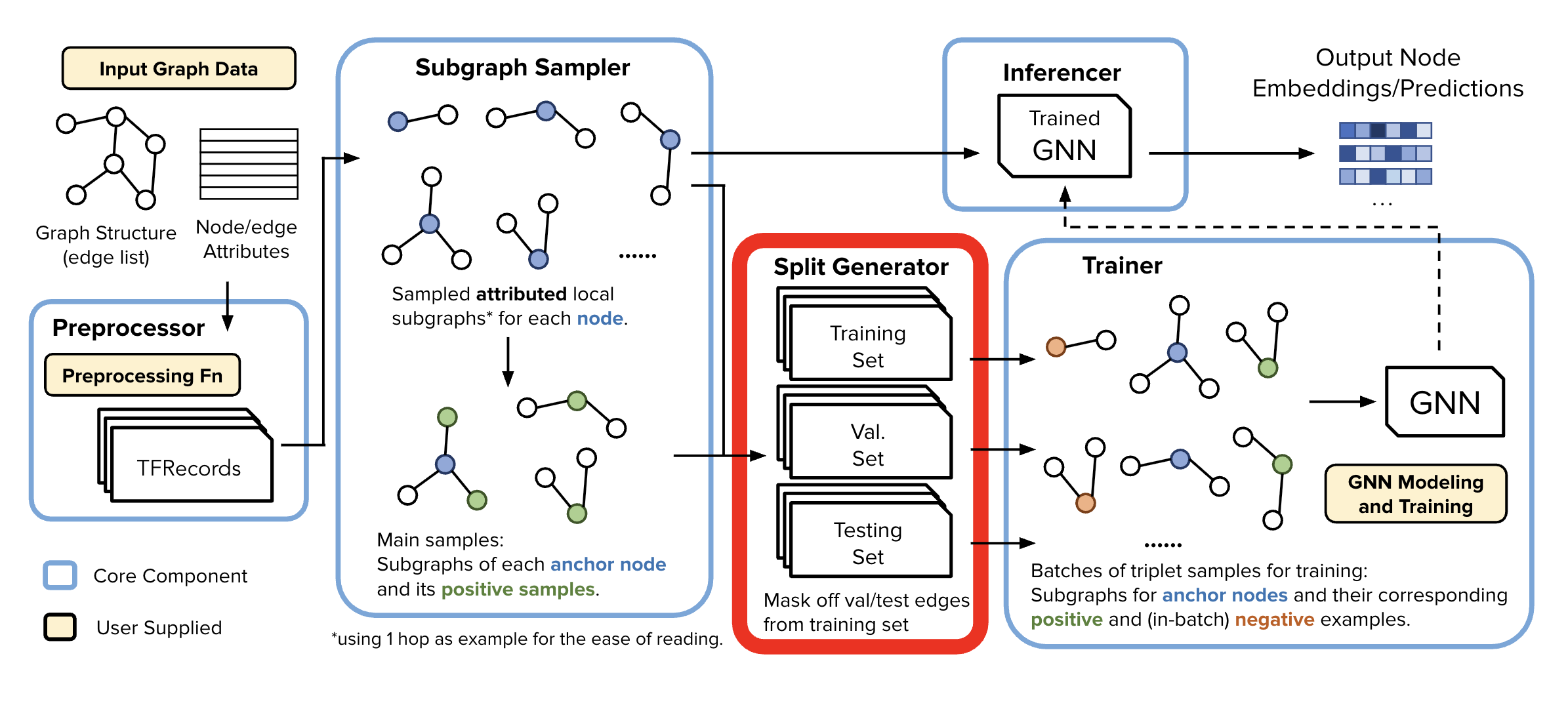
Split Generator#
Generating Train/Test/Val Splits
print(frozen_task_config.dataset_config.split_generator_config)
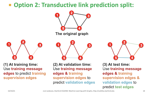
🔀 Split Strategy: Transductive#
In this example, we’re using the transductive split strategy, as specified in the frozen_config. For transductive, at training time, it uses training message edges to predict training supervision edges. At validation time, the training message edges and training supervision edges are used to predict the validation edges and then all 3 are used to predict test edges.
📦 Role of the Split Generator#
The Split Generator reads localized subgraph samples produced by the SGS and applies the selected SplitStrategy to divide the data into: train/val/test splits
🧩 Supported Split Strategies (GiGL Platform)#
Several standard split routines are implemented and available via SplitStrategy and Assigner classes, including:
Inductive Node Classification
Transductive Node Classification
Transductive Link Prediction
📚 Further Reading#
To understand the theory behind these strategies, see:
Graph Link Prediction (relevant for explaining transductive vs inductive).
!python -m gigl.src.split_generator.split_generator \
--job_name=$JOB_NAME \
--task_config_uri=$FROZEN_TASK_CONFIG_PATH \
--resource_config_uri=$RESOURCE_CONFIG_PATH
Upon completion, there will be 3 folders for train,test, and val. Each of them contains the protos for the positive and negaitve samples. The path for these folders is specified in the following location in the frozen_config:
dataset_metadata = frozen_task_config.shared_config.dataset_metadata
print(dataset_metadata)
🖼️ Visualizing Samples#
We will visualize the train, validation, and test samples for a few nodes. These subgraphs are generated based on the configured task setup.
⚠️ Important Note on Validation & Test Sets: Due to the way edges are randomly bucketed into train, val, and test sets—independent of their status as supervision (i.e., labeled) edges, not all validation or test samples will contain positive labels.
This behavior is intentional and acceptable at scale. When working with large datasets and large batch sizes, it’s statistically likely that each batch will contain some supervision edges. However, individual batches may occasionally lack them, especially in val/test.
🧠 Implications for Training#
This design introduces some considerations:
✅ Training samples are typically unaffected due to the high frequency of labeled edges.
⚠️ Although, at large scale it is not frequent, validation and test Loops need to account for batches without any supervision edges.
🛑 Early Stopping Logic should be robust to these fluctuations e.g., don’t trigger early stopping based on a single underperforming batch.
from gigl.common.utils.jupyter_magics import GraphVisualizerLayoutMode

for node_id in range(min(original_graph_heterodata.num_nodes, 2)):
    print(f"Node anchor prediction sample for node {node_id}:")
    sample_train = pb_visualizer.find_node_pb(
        from_output=PbVisualizerFromOutput.SPLIT_TRAIN,
        unenumerated_node_id=node_id,
        unenumerated_node_type="user",
        pb_type=training_samples_schema_pb2.NodeAnchorBasedLinkPredictionSample,
    )
    sample_val = pb_visualizer.find_node_pb(
        from_output=PbVisualizerFromOutput.SPLIT_VAL,
        unenumerated_node_id=node_id,
        unenumerated_node_type="user",
        pb_type=training_samples_schema_pb2.NodeAnchorBasedLinkPredictionSample,
    )
    sample_test = pb_visualizer.find_node_pb(
        from_output=PbVisualizerFromOutput.SPLIT_TEST,
        unenumerated_node_id=node_id,
        unenumerated_node_type="user",
        pb_type=training_samples_schema_pb2.NodeAnchorBasedLinkPredictionSample,
    )
    if sample_train:
        print(f"Train sample for node {node_id}: ")
        pb_visualizer.plot_pb(
            sample_train,
            layout_mode=GraphVisualizerLayoutMode.HOMOGENEOUS,
        )
    else:
        print(f"No train sample found for node {node_id}.")
    if sample_val:
        print(f"Validation sample for node {node_id}:")
        pb_visualizer.plot_pb(
            sample_val,
            layout_mode=GraphVisualizerLayoutMode.HOMOGENEOUS,
        )
    else:
        print(f"No validation sample found for node {node_id}.")
    if sample_test:
        print(f"Test sample for node {node_id}:")
        pb_visualizer.plot_pb(
            sample_test,
            layout_mode=GraphVisualizerLayoutMode.HOMOGENEOUS,
        )
    else:
        print(f"No test sample found for node {node_id}.")
At this point, we have our graph data samples ready to be processed by the trainer and inferencer components. These components will extract representations/embeddings by learning contextual information for the specified task.
Training and Inference#
!python -m gigl.src.training.trainer \
--job_name=$JOB_NAME \
--task_config_uri=$FROZEN_TASK_CONFIG_PATH \
--resource_config_uri=$RESOURCE_CONFIG_PATH \
--cpu_docker_uri=$CPU_SRC_IMG \
--cuda_docker_uri=$CUDA_SRC_IMG
# The model gets saved to the path specified in the frozen task config.
print(
    f"Trained model saved to: {frozen_task_config.shared_config.trained_model_metadata.trained_model_uri}"
)
!python -m gigl.src.inference.inferencer \
--job_name=$JOB_NAME \
--task_config_uri=$FROZEN_TASK_CONFIG_PATH \
--resource_config_uri=$RESOURCE_CONFIG_PATH \
--cpu_docker_uri=$CPU_SRC_IMG \
--cuda_docker_uri=$CUDA_SRC_IMG \
--custom_worker_image_uri=$DATAFLOW_RUNTIME_IMG
# Looking at inference results

from gigl.src.common.utils.bq import BqUtils

bq_emb_out_table = frozen_task_config.shared_config.inference_metadata.node_type_to_inferencer_output_info_map[
    frozen_task_config.graph_metadata_pb_wrapper.homogeneous_node_type
].embeddings_path
print(
    f"Embeddings should be successfully stored in the following location: {bq_emb_out_table}"
)

bq_utils = BqUtils(project=resource_config.project)
query = f"SELECT * FROM {bq_emb_out_table} LIMIT 5"
result = list(bq_utils.run_query(query=query, labels={}))

print(f"Query result: ")
for row in result:
    print(row)
Vertex AI Pipelines#
You can also run GiGL pipelines on Vertex AI Pipelines. Doing so provides a number of advantages, such as:
Decoupling orchestration from dev machines - when you close your laptop the pipeline keeps running
Orchestrate new runs from GCP console. You can start/stop runs on the console
Data isolation - production Service Accounts and Projects can access sensitive data
GiGL has a KfpOrchestrator client which will let you launch GiGL pipelines on Vertex AI.
We need to call two methods on the client to start a new pipeline run:
compile, which generates a KFP Pipeline spec that Vertex AI can consume to orchestrate the pipeline. Under the hood, we write the pipeline yaml to some local file, but you can configure this with thedst_compiled_pipeline_pathargument.runwhich uploads the pipeline spec to Vertex AI and starts a new pipeline job. Note thatrunrequires an applied_task_identifier (pipeline job name), which must be unique in every Project and Region.
Note that compile requires docker images to be passed in, this is because the docker images that are used by each component are baked into the pipeline definition. For this tutorial, we will be using the default images, however if you want to customize the buisness logic here, you will need to provide your own docker images. GiGL has a handy script will push the docker images for you.
# You can also run the entire GiGL pipeline on Vertex AI
# With the KfpOrchestrator [1]
# Note that we use TEMPLATE_TASK_CONFIG_PATH here so we can have another "dataset" e.g. SharedConfig.
# [1]: https://snapchat.github.io/GiGL/docs/api/gigl/orchestration/kubeflow/kfp_orchestrator/index.html#gigl.orchestration.kubeflow.kfp_orchestrator.KfpOrchestrator
from gigl.orchestration.kubeflow.kfp_orchestrator import KfpOrchestrator

orchestrator = KfpOrchestrator()
# First, compile the KFP pipeline definition
orchestrator.compile(
    cuda_container_image=CUDA_SRC_IMG,
    cpu_container_image=CPU_SRC_IMG,
    dataflow_container_image=DATAFLOW_RUNTIME_IMG,
)
# Then, run it.
orchestrator.run(
    applied_task_identifier=JOB_NAME,
    task_config_uri=TEMPLATE_TASK_CONFIG_PATH,
    resource_config_uri=RESOURCE_CONFIG_PATH,
)

# You'll eventually see a link to the KFP pipeline in the logs.
# Something like:
# https://console.cloud.google.com/vertex-ai/pipelines/locations/us-central1/runs/<job_id>